Complexity Analysis

We can assess the efficiency of an algorithm in terms of space and time, without actually running it and yet understand how slow/fast it is.

The complexity of an algorithm is denoted with the Big O notation, which describes the limiting behavior of a certain function when the argument tends to a particular value or infinity [1].

Classes of Functions

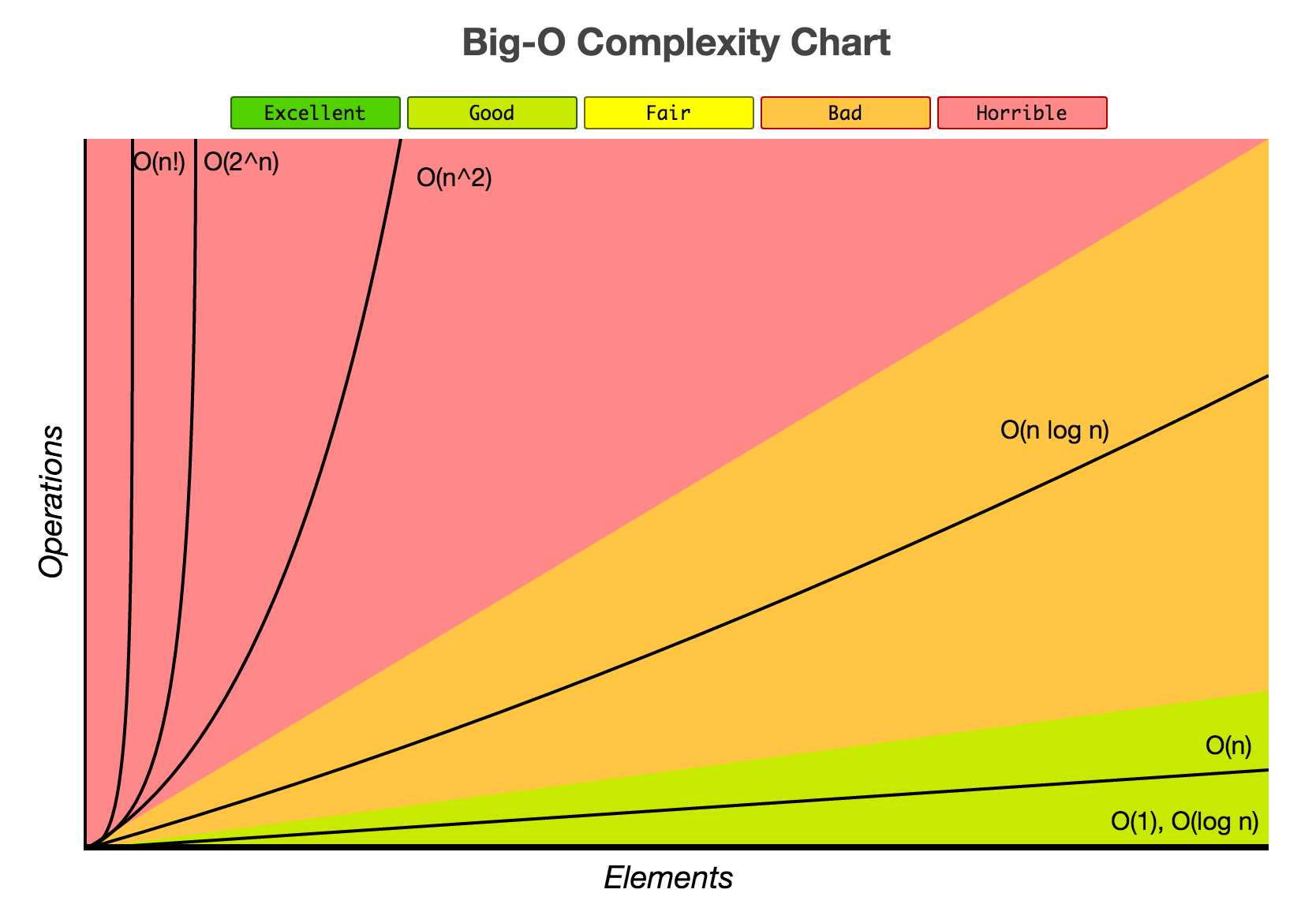
Before explaining how to measure the efficiency of an algorithm, we have to understand how to compare functions bounded to an input $n$ .

In fact, since both time and space complexities are expressed through mathematical functions, we need a way to compare them.

This chart [2] will help us:

Big O complexity chart. *Chart by bigocheatsheet.com.*

You will likely found $n$ somewhere inside this $O$ notation (e.g. $O (n)$ ), but $n$ is just the name of a variable. You can use any name you want, but, of course, $n$ is the most common to indicate the size of a certain input.

However, nothing prevents you to use other names. Just keep in mind that you have to pay attention on how you map the name of a certain variable to the inputs of your algorithm.

For example, you can use $n$ to map the size of a list. However, you could also use $m$ , $x$ , $y$ , or your preferred variable's name.

Common complexities

Before looking at some examples, remember that constant values are not considered. So, for example, $O (2 n)$ and $O (10 + n)$ are both $O (n)$ .

Moreover, we are also going to ignore terms with the lowest growth rate: $O (n^{2} + n)$ is just $O (n^{2})$ .

Constant time

It is indicated with $O (1)$ . Some examples:

# mathematical operations
a = 1
b = 2
c = a + b

# sets/hash-maps lookup
1 in s  # where `s = {1, 2, 3}`
2 in map  # where `m = {1: "one", 2: "two", 3: "three"}`

# pushing/popping from a stack
s = []
s.append(1)
s.append(2)
s.pop()

# enqueuing/dequeuing from a double-ended queue
from collections import deque
q = deque()
q.append(1)
q.append(2)
q.popleft()

Logarithmic time

It is indicated with $O (l o g (n))$ . This is common for the Binary Search algorithm, and, more generally, whenever the search space is halved at each iteration.

Linear time

It is indicated with $O (n)$ . This is probably the most common one, especially if the algorithm uses loops bounded to the size of the input.

The following are all $O (n)$ algorithms. Even with nested loops, we can still have such linear complexity. Just be careful on the used variables.

nums: List[Any] = ...  # a list took as input

# traverse a list (simplest case)
for num in nums:
    print(num)


# two nested loop, but `m` is a constant
m = 2
for num in nums:
    for _ in range(m):
        print(num)


# two consecutive loops: `O(2 * n)`, hence `O(n)`
for num in nums:
    print(num)

for num in nums:
    print(num)
# ~


# find an element in a list. In the worst case, you need to traverse the entire list
target = 10
for num in nums:
    if num == target:
        print(f"Found the target `{target}`")
        break

Logarithmic time with constant operations

It is indicated with $O (c l o g (n))$ , where $c$ is a constant factor.

You will usually encounter this complexity after applying a logarithmic algorithm for $c$ times. Some examples are Binary Search and push/pop operations in a Heap.

Linearithmic time (Linear * Logarithmic)

It is indicated with $O (n l o g (n))$ .

You will usually encounter this complexity for sorting algorithms, and divide and conquer ones.

Quadratic time

It is indicated with $O (n^{2})$ . Some examples:

# traverse a quadratic matrix
matrix: List[List[Any]] = ...  # a quadratic matrix took as input
n = len(nums)
for i in range(n):
    for j in range(n):
        print(matrix[i][j])


# traverse a list twice
nums: List[Any] = ...  # a list took as input
n = len(nums)
for i in range(n):
    for j in range(i, n):
        pass

algo-ds.com

Complexity Analysis

Classes of Functions

The importance of $n$